Polar Ice Page Update

So I updated the polar sea ice page once again. Note the ever growing area of sea ice on the Southern hemisphere.

PDF to animated GIF

In order to illustrate how fragmentation occurs, I created a PDF document (Fragmentierung.pdf) with one page for each step of the fragmentation.

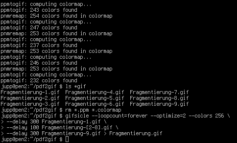
 This is how I converted it to an animated GIF. The first step was to create a series of PPM files, one file for each page. The option -r 384 sets the resolution to 384 dpi. This somewhat odd resolution is four times 96 dpi which in turn is the resolution of the PDF being converted.

The pdftoppm command generates files that are numbered.

The files resulting from this conversation are huge in both display and storage size so the next step is to rescale them to a reasonable resolution. My choice was a width of 800 times 600. the for loop iterates over all PPM files, the output of the pamscale command sent to a file with a name based on the original file name using the shell's own capability to process strings. Finally, the --filter option controls how precisely the original high-resolution image is mapped to the low resolution one.

Let's assume the original file name is Fragmentierung-1.ppm. Then ${i%.ppm} yields Fragmentierung-1 and ${i%.ppm}_new.ppm results in Fragmentierung-1_new.ppm.

The result of this command - which on my old machine requires a considerable amount of time - is a new series of files that are considerably smaller than the original ones.

As the old files are no longer needed, I replace them with the corresponding new ones.

Now we have ppm files of the right size that are simply numbered.

The PPM files usually have more than 256 colors (which is the maximum for GIFs). For this reason I use pnmcolormap to generate colormaps for the individual files that have no more than 256 colors.

This command results in tons of diagnostics output created by pnmcolormap.

The next command performs two tasks at the same time: pnmremap uses the colormap to map the original colors to no more than 256 with the -fs option making sure that Floyd-Steinberg dithering is used. Then the output converted to GIF formatusing ppmtogif and is written to a file with the file name extension .gif.

In this case both commands are a bit chatty so you again get lots of output.

Now we are almost done as we have a set of GIF files.

Just discard all the intermediary files. The next command looks complicated like hell but it isn't. gifsicle generates an animated GIF from a number of input files that need to be in GIF format.

• --loopcount=forever makes the animation loop forever (i.e. after displaying the last frame of the animation it always restarts with the first one)
• --optimize=2 optimizes the generated file as much as possible (without this option the file gets even bigger)
• --colors=256 makes sure that the generated file has no more than 256 colors. This may seem superflous as each input file already has no more than 256 colors but the colors may happen to be different so that the overall number can be larger than 256.

The most important part of the command is the --delay options. If you provide this option, it applies to each image that follows up to the next command. Hence, in this case the first delay of 3 seconds applies to Fragmentierung-1.gif only, the delay of 1 seconds to Fragmentierung-2.gif through Fragmentierung-8.gif and the second delay of 3 seconds to Fragmentierung-9.gif.

Finally done. Here is the animated gif that results from this effort.

Katyusha (Катюша)

I am a huge fan of Igor Presnyakov and what he does to/with his acoustic guitar.

Hear him perform the Russian song Katyusha (Катюша)

Distances from Bonn

I came up with the strange idea of sorting European capitals by how far they are from the town I live in (Bonn, Germany) and found that half a dozen of foreign capitals are nearer than the capital of Germany.

City	Country	Distance in km
Luxembourg City	Luxembourg	142
City of Brussels	Belgium	195
Amsterdam	Netherlands	234
Paris	France	400
Bern	Switzerland	425
Vaduz	Liechtenstein	437
Berlin	Germany	478
London	United Kingdom	510
Prague	Czech Republic	527
Copenhagen	Denmark	659
Vienna	Austria	726
Ljubljana	Slovenia	755
Bratislava	Slovakia	779
Monaco	Monaco	779
City of San Marino	San Marino	857
Zagreb	Croatia	857
Budapest	Hungary	942
Dublin	Republic of Ireland	957
Warsaw	Poland	976
Oslo	Norway	1047
Rome	Italy	1065
Vatican City	Vatican City	1065
Sarajevo	Bosnia and Herzegovina	1143
Stockholm	Sweden	1181
Belgrade	Serbia	1195
Vilnius	Lithuania	1300
Riga	Latvia	1308
Podgorica	Montenegro	1347
Madrid	Spain	1421
Minsk	Belarus	1430
Tirana	Albania	1432
Ankara	Turkey	1447
Skopje	Macedonia	1463
Tallinn	Estonia	1474
Sofia	Bulgaria	1522
Helsinki	Finland	1530
Bucharest	Romania	1583
Chişinău	Moldova	1639
Kiev	Ukraine	1648
Valletta	Malta	1745
Lisbon	Portugal	1845
Athens	Greece	1931
Moscow	Russia	2086
Reykjavík	Iceland	2257
Tbilisi	Georgia	3034
Yerevan	Armenia	3106
Baku	Azerbaijan	3469

If you find this idea interesting what about composing a similar table for the location you live in?

Obtaining Tweeted Images in Original Size

An increasing number of tweets contains images uploded to twitter. Here is one example:

A particular example

I assume that you know how to find out URLs of images that are used on a web page.

The URL of the image you see in the tweet is https://pbs.twimg.com/media/A0BRGqGCcAEBdHW.jpg with the dimensions 600px × 428px (scaled to 435px × 310px).

If you click on the image to obtain a larger version you are presented with https://pbs.twimg.com/media/A0BRGqGCcAEBdHW.jpg:large with the dimensions 1,024px × 730px. This still isn't the original image.

I then made a well-educated guess and tried
https://pbs.twimg.com/media/A0BRGqGCcAEBdHW.jpg:orig and it actually worked; I got the original size image with dimensions 2,048px × 1,460px.

So all you need to do to obtain an original size image is to append »:orig« to the URL of the small version of the image.

Note that this only works for images uploaded to twitter not for images hosted on flickr.

Here is one example: https://twitter.com/VirtualAstro/status/241683461155475456 shows a nice photo of a blue moon; the 3 MP image can be found at https://pbs.twimg.com/media/A1qS3JvCQAE0QPv.jpg:orig

Polar Sea Ice Page Updated

I had to update the Polar Sea Ice page because it referred to the record ice extent as data of 2007 while in reality the record extents (minimum in the Arctic, maximum in the Antarctic) are currently being updated every day (as of writing this on 2012-09-02).

I originally did not expect this to become necessary so soon. The reason for this misjudgement of mine is the Atlantic Multi-decadal Oscillation. Back in 2008 I learned that it should currently be counteracting the effect of global warming on the Arctic region.

A BBC article of 2008-05-01 puts it like that:

The Earth's temperature may stay roughly the same for a decade, as natural climate cycles enter a cooling phase … A new computer model … suggests the cooling will counter greenhouse warming. However, temperatures will again be rising quickly by about 2020 …

In contrast, a recent BBC article (2012-08-27) has this to say:

A recent paper from Reading University … [estimated] that between 5-30% of the recent ice loss was due to Atlantic Multi-decadal Oscillation - a natural climate cycle repeating every 65-80 years. It's been in warm phase since the mid 1970s.

Allow me to call this difference in description a little strange.

NASA: Arctic sea ice reaches record low

Asteroids Missing Earth: What Means “Close Call”?

Every now and then you read about asteroids passing Earth in a certain distance but nobody gives you a feeling of how close such an encounter is. Allow me to fill in this gap.

Say an asteroid passes in a distance x from Earth, the radius of which we will call r. We now can ask how likely it is that an object that hits a disk of radius r+x also hits a disk of radius r provided that it any point on the larger disk is hit with equal likelihood.

The likelihood then is p = A(r)/A(r+x) where A is the area of a disk of the given radius, In other words p = πr²/π(r+x)² = 1/(1+x/r)². If we now define ξ=x/r (which is the distance in units of Earth's radius we get a quite simple formula: p = 1/(1+ξ)².

Using ξ is advantageous as it is a value you actually find in tables. Let’s try a couple of values; LD means Lunar distance and is the distance in terms of the average distance between Earth and Moon:

Distance in		ξ	p in %
LD	km
1.65614	636619.77	100	0.098
0.49684	190985.93	30	0.104
0.16561	63661.98	10	0.826
0.04968	19098.59	3	6.250
0.01656	6366.20	1	25.000
0.00497	1909.86	0.3	59.172
0.00166	636.62	0.1	82.645
0.00050	190.99	0.03	94.260
0.00017	63.66	0.01	98.030

Please note that the closer an encounter is the less meaningless this rough estimate becomes as the asteroid by no means randomly hits the disk of radius r+x but follows a clearly determined path.